Use case example: Evolution of Sovereignty Attitudes

This page uses the merged file to estimate sovereignty support over time.

Show code used in this page

library(dplyr)
library(ggplot2)
library(knitr)

pkg_master <- system.file("extdata", "qes_master.csv", package = "qesR")
master_paths <- c("qes_master.csv", "../qes_master.csv", pkg_master)
master_paths <- master_paths[nzchar(master_paths)]
master <- read.csv(master_paths[file.exists(master_paths)][1], stringsAsFactors = FALSE)

master <- master %>%
  mutate(
    qes_year_chr = trimws(as.character(qes_year)),
    qes_year_num = as.integer(substr(qes_year_chr, 1, 4))
  )

is_range <- grepl("^[0-9]{4}-[0-9]{4}$", master$qes_year_chr)
start_year <- suppressWarnings(as.numeric(sub("^([0-9]{4})-([0-9]{4})$", "\\1", master$qes_year_chr)))
end_year <- suppressWarnings(as.numeric(sub("^([0-9]{4})-([0-9]{4})$", "\\2", master$qes_year_chr)))

master$study_period <- ifelse(
  is_range,
  master$qes_year_chr,
  ifelse(!is.na(master$qes_year_num), as.character(master$qes_year_num), master$qes_year_chr)
)
master$period_order <- ifelse(
  is_range & is.finite(start_year) & is.finite(end_year),
  (start_year + end_year) / 2,
  master$qes_year_num
)

master$sovereignty_support <- suppressWarnings(as.numeric(master$sovereignty_support))
master$sovereignty_support[!(master$sovereignty_support %in% c(0, 1))] <- NA_real_

all_periods <- master %>%
  filter(!is.na(study_period), nzchar(study_period), !is.na(period_order)) %>%
  distinct(study_period, period_order)

sov <- master %>%
  filter(!is.na(study_period), nzchar(study_period), !is.na(period_order)) %>%
  group_by(study_period, period_order) %>%
  summarise(
    respondents = n(),
    n_with_measure = sum(!is.na(sovereignty_support)),
    support_share = ifelse(n_with_measure > 0, mean(sovereignty_support, na.rm = TRUE), NA_real_),
    se = ifelse(n_with_measure > 0, sqrt(pmax(support_share * (1 - support_share), 0) / n_with_measure), NA_real_),
    ci_low = ifelse(!is.na(se), pmax(0, support_share - 1.96 * se), NA_real_),
    ci_high = ifelse(!is.na(se), pmin(1, support_share + 1.96 * se), NA_real_),
    .groups = "drop"
  )

sov <- merge(all_periods, sov, by = c("study_period", "period_order"), all.x = TRUE, sort = TRUE)
sov <- sov %>% arrange(period_order, study_period)
sov$period_index <- seq_len(nrow(sov))

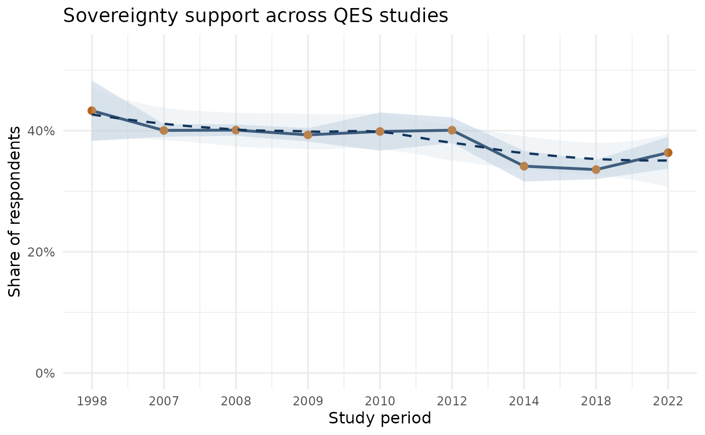
knitr::kable(sov)

The estimates below use the dedicated sovereignty question harmonized across study periods.

Table 1: sovereignty support by study period

Sovereignty support by study period

Study period	N respondents	N with sovereignty item	Sovereignty support (%)	95% CI (%)
1998	1483	381	43.3	38.3 to 48.3
2007	9244	8207	40.1	39.0 to 41.1
2008	11162	10379	40.1	39.2 to 41.0
2009	8008	7455	39.3	38.2 to 40.4
2010	1000	923	39.9	36.7 to 43.0
2012	2349	2066	40.1	38.0 to 42.2
2014	1517	1353	34.1	31.6 to 36.7
2018	4322	3338	33.6	32.0 to 35.2
2022	1521	1284	36.4	33.7 to 39.0

Figure 1: sovereignty trend

Notes

• The sovereignty trend uses the dedicated sovereignty item from each study.
• The qes_crop_2007_2010 study is split into 2007, 2008, 2009, and 2010 using its collection-wave date variable.
• Confidence intervals are binomial 95% intervals using normal approximation.
• n_with_measure in the table shows where coverage is thinner.